Neurons and Layers

Neurons and Layers

This lab is about basic understanding of neuron & layers. Use of them through tensorflow and keras.

This Neurons and Layers is part of DeepLearning.AI course: Machine Learning Specialization / Course 2: Advanced Learning Algorithms: Neural Network Model You will build and train a neural network with TensorFlow to perform multi-class classification in the second course of the Machine Learning Specialization. Ensure that your machine learning models are generalizable by applying best practices for machine learning development. You will build and train a neural network using TensorFlow to perform multi-class classification in the second course of the Machine Learning Specialization. Implement best practices for machine learning development to ensure that your models are generalizable to real-world data and tasks. Create and use decision trees and tree ensemble methods, including random forests and boosted trees.

This is my learning experience of data science through DeepLearning.AI. These repository contributions are part of my learning journey through my graduate program masters of applied data sciences (MADS) at University Of Michigan, DeepLearning.AI, Coursera & DataCamp. You can find my similar articles & more stories at my medium & LinkedIn profile. I am available at kaggle & github blogs & github repos. Thank you for your motivation, support & valuable feedback.

These include projects, coursework & notebook which I learned through my data science journey. They are created for reproducible & future reference purpose only. All source code, slides or screenshot are intellectual property of respective content authors. If you find these contents beneficial, kindly consider learning subscription from DeepLearning.AI Subscription, Coursera, DataCamp

Optional Lab - Neurons and Layers

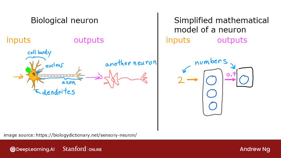
In this lab we will explore the inner workings of neurons/units and layers. In particular, the lab will draw parallels to the models you have mastered in Course 1, the regression/linear model and the logistic model. The lab will introduce Tensorflow and demonstrate how these models are implemented in that framework.

Packages

Tensorflow and Keras Tensorflow is a machine learning package developed by Google. In 2019, Google integrated Keras into Tensorflow and released Tensorflow 2.0. Keras is a framework developed independently by François Chollet that creates a simple, layer-centric interface to Tensorflow. This course will be using the Keras interface.

import numpy as np
import matplotlib.pyplot as plt
import tensorflow as tf
from tensorflow.keras.layers import Dense, Input
from tensorflow.keras import Sequential
from tensorflow.keras.losses import MeanSquaredError, BinaryCrossentropy
from tensorflow.keras.activations import sigmoid
from lab_utils_common import dlc
from lab_neurons_utils import plt_prob_1d, sigmoidnp, plt_linear, plt_logistic
plt.style.use('deeplearning.mplstyle')
import logging
logging.getLogger("tensorflow").setLevel(logging.ERROR)
tf.autograph.set_verbosity(0)

Neuron without activation - Regression/Linear Model

DataSet

We’ll use an example from Course 1, linear regression on house prices.

X_train = np.array([[1.0], [2.0]], dtype=np.float32)           #(size in 1000 square feet)
Y_train = np.array([[300.0], [500.0]], dtype=np.float32)       #(price in 1000s of dollars)

fig, ax = plt.subplots(1,1)
ax.scatter(X_train, Y_train, marker='x', c='r', label="Data Points")
ax.legend( fontsize='xx-large')
ax.set_ylabel('Price (in 1000s of dollars)', fontsize='xx-large')
ax.set_xlabel('Size (1000 sqft)', fontsize='xx-large')
plt.show()

Regression/Linear Model

The function implemented by a neuron with no activation is the same as in Course 1, linear regression: \[ f_{\mathbf{w},b}(x^{(i)}) = \mathbf{w}\cdot x^{(i)} + b \tag{1}\]

We can define a layer with one neuron or unit and compare it to the familiar linear regression function.

linear_layer = tf.keras.layers.Dense(units=1, activation = 'linear', )

Let’s examine the weights.

linear_layer.get_weights()

[]

There are no weights as the weights are not yet instantiated. Let’s try the model on one example in X_train. This will trigger the instantiation of the weights. Note, the input to the layer must be 2-D, so we’ll reshape it.

a1 = linear_layer(X_train[0].reshape(1,1))
print(a1)

tf.Tensor([[1.09]], shape=(1, 1), dtype=float32)

The result is a tensor (another name for an array) with a shape of (1,1) or one entry. Now let’s look at the weights and bias. These weights are randomly initialized to small numbers and the bias defaults to being initialized to zero.

w, b= linear_layer.get_weights()
print(f"w = {w}, b={b}")

w = [[1.09]], b=[0.]

A linear regression model (1) with a single input feature will have a single weight and bias. This matches the dimensions of our linear_layer above.

The weights are initialized to random values so let’s set them to some known values.

set_w = np.array([[200]])
set_b = np.array([100])

# set_weights takes a list of numpy arrays
linear_layer.set_weights([set_w, set_b])
print(linear_layer.get_weights())

[array([[200.]], dtype=float32), array([100.], dtype=float32)]

Let’s compare equation (1) to the layer output.

a1 = linear_layer(X_train[0].reshape(1,1))
print(a1)
alin = np.dot(set_w,X_train[0].reshape(1,1)) + set_b
print(alin)

tf.Tensor([[300.]], shape=(1, 1), dtype=float32)
[[300.]]

They produce the same values! Now, we can use our linear layer to make predictions on our training data.

prediction_tf = linear_layer(X_train)
prediction_np = np.dot( X_train, set_w) + set_b

plt_linear(X_train, Y_train, prediction_tf, prediction_np)

Neuron with Sigmoid activation

The function implemented by a neuron/unit with a sigmoid activation is the same as in Course 1, logistic regression: \[ f_{\mathbf{w},b}(x^{(i)}) = g(\mathbf{w}x^{(i)} + b) \tag{2}\] where \[g(x) = sigmoid(x)\]

Let’s set \(w\) and \(b\) to some known values and check the model.

DataSet

We’ll use an example from Course 1, logistic regression.

X_train = np.array([0., 1, 2, 3, 4, 5], dtype=np.float32).reshape(-1,1)  # 2-D Matrix
Y_train = np.array([0,  0, 0, 1, 1, 1], dtype=np.float32).reshape(-1,1)  # 2-D Matrix

pos = Y_train == 1
neg = Y_train == 0
X_train[pos]

array([3., 4., 5.], dtype=float32)

pos = Y_train == 1
neg = Y_train == 0

fig,ax = plt.subplots(1,1,figsize=(4,3))
ax.scatter(X_train[pos], Y_train[pos], marker='x', s=80, c = 'red', label="y=1")
ax.scatter(X_train[neg], Y_train[neg], marker='o', s=100, label="y=0", facecolors='none',
              edgecolors=dlc["dlblue"],lw=3)

ax.set_ylim(-0.08,1.1)
ax.set_ylabel('y', fontsize=12)
ax.set_xlabel('x', fontsize=12)
ax.set_title('one variable plot')
ax.legend(fontsize=12)
plt.show()

Logistic Neuron

We can implement a ‘logistic neuron’ by adding a sigmoid activation. The function of the neuron is then described by (2) above. This section will create a Tensorflow Model that contains our logistic layer to demonstrate an alternate method of creating models. Tensorflow is most often used to create multi-layer models. The Sequential model is a convenient means of constructing these models.

model = Sequential(
    [
        tf.keras.layers.Dense(1, input_dim=1,  activation = 'sigmoid', name='L1')
    ]
)

model.summary() shows the layers and number of parameters in the model. There is only one layer in this model and that layer has only one unit. The unit has two parameters, \(w\) and \(b\).

model.summary()

Model: "sequential_1"
_________________________________________________________________
 Layer (type)                Output Shape              Param #   
=================================================================
 L1 (Dense)                  (None, 1)                 2         
                                                                 
=================================================================
Total params: 2
Trainable params: 2
Non-trainable params: 0
_________________________________________________________________

logistic_layer = model.get_layer('L1')
w,b = logistic_layer.get_weights()
print(w,b)
print(w.shape,b.shape)

[[1.29]] [0.]
(1, 1) (1,)

set_w = np.array([[2]])
set_b = np.array([-4.5])
# set_weights takes a list of numpy arrays
logistic_layer.set_weights([set_w, set_b])
print(logistic_layer.get_weights())

[array([[2.]], dtype=float32), array([-4.5], dtype=float32)]

Let’s compare equation (2) to the layer output.

a1 = model.predict(X_train[0].reshape(1,1))
print(a1)
alog = sigmoidnp(np.dot(set_w,X_train[0].reshape(1,1)) + set_b)
print(alog)

1/1 [==============================] - 0s 18ms/step
[[0.01]]
[[0.01]]

They produce the same values! Now, we can use our logistic layer and NumPy model to make predictions on our training data.

plt_logistic(X_train, Y_train, model, set_w, set_b, pos, neg)

1/1 [==============================] - 0s 7ms/step
1/1 [==============================] - 0s 7ms/step
1/1 [==============================] - 0s 7ms/step
1/1 [==============================] - 0s 7ms/step
1/1 [==============================] - 0s 7ms/step
1/1 [==============================] - 0s 7ms/step
1/1 [==============================] - 0s 7ms/step
1/1 [==============================] - 0s 7ms/step
1/1 [==============================] - 0s 7ms/step
1/1 [==============================] - 0s 7ms/step
1/1 [==============================] - 0s 8ms/step
1/1 [==============================] - 0s 8ms/step
1/1 [==============================] - 0s 7ms/step
1/1 [==============================] - 0s 7ms/step
1/1 [==============================] - 0s 7ms/step
1/1 [==============================] - 0s 7ms/step
1/1 [==============================] - 0s 7ms/step
1/1 [==============================] - 0s 7ms/step
1/1 [==============================] - 0s 7ms/step
1/1 [==============================] - 0s 7ms/step
1/1 [==============================] - 0s 7ms/step
1/1 [==============================] - 0s 7ms/step
1/1 [==============================] - 0s 7ms/step
1/1 [==============================] - 0s 7ms/step
1/1 [==============================] - 0s 8ms/step
1/1 [==============================] - 0s 7ms/step
1/1 [==============================] - 0s 7ms/step
1/1 [==============================] - 0s 7ms/step
1/1 [==============================] - 0s 7ms/step
1/1 [==============================] - 0s 7ms/step
1/1 [==============================] - 0s 7ms/step
1/1 [==============================] - 0s 7ms/step
1/1 [==============================] - 0s 7ms/step
1/1 [==============================] - 0s 7ms/step
1/1 [==============================] - 0s 7ms/step
1/1 [==============================] - 0s 7ms/step
1/1 [==============================] - 0s 7ms/step
1/1 [==============================] - 0s 7ms/step
1/1 [==============================] - 0s 7ms/step
1/1 [==============================] - 0s 7ms/step
1/1 [==============================] - 0s 7ms/step
1/1 [==============================] - 0s 7ms/step
1/1 [==============================] - 0s 7ms/step
1/1 [==============================] - 0s 7ms/step
1/1 [==============================] - 0s 6ms/step
1/1 [==============================] - 0s 7ms/step
1/1 [==============================] - 0s 8ms/step
1/1 [==============================] - 0s 7ms/step
1/1 [==============================] - 0s 8ms/step
1/1 [==============================] - 0s 7ms/step

The shading above reflects the output of the sigmoid which varies from 0 to 1.